
1. The FPCUP SNOWLOADS project
The FPCUP project started in July 2018 and is led by the German Aerospace Center (DLR) and funded by the European Commission (DG DEFIS) responding on an EU call to establish the Caroline Herschel Framework Partnership Agreement between the Commission and Copernicus Participating States. Thus, FPCUP is one specific part in the Commissions’ User Uptake Strategy setting up a Framework Partnership Agreement (FPA) for user uptake with Member States. The FPCUP project's general objectives are to promote the use of earth observation in applications and services, in order to develop a competitive European space and service industry which is key for Europe to achieve independent decision-making and action. The joint action by the FPCUP internal Working Group “Snowloads” started in October 2020. This is a collaboration with partners from Deutscher Wetterdienst (DWD), Centre national de la recherche scientifique (CNRS), Finnish Meteorological Institute (FMI) and Politecnico di Milano (POLIMI) that addresses the development of a dedicated online visualization App based on Copernicus Climate Change Service (C3S) data for a Europe-wide provision of snow load climatological information for civil engineering as well as hazard and damage prevention purposes. This App is referred to as the FPCUP “snowload” C3S App. Three pilot downstream services will use the data of the C3S App as basic and background information on snow loads and will enrich them with current snow load information in the pilot regions Bavaria (Germany), Uusimaa (Finland) and Lombardia (Italy).
2. The FPCUP 'snowload' C3S App
This portal provides information about present and future 50-year return level estimations of maximum annual snow mass, as these are key values of the second generation of Eurocodes FprEN 1991-1-3:2024 'Actions on structures: Snow loads'. Estimations are based on datasets of regional reanalyses and regional climate projections from C3S. It enables users to visualize regional data depending on elevation and location. The current portal is for demonstration only, and may later be implemented directly on a Copernicus-hosted portal. We describe here the parameters to be tuned by each user, and the resulting output provided by the application.
3. User inputs and options
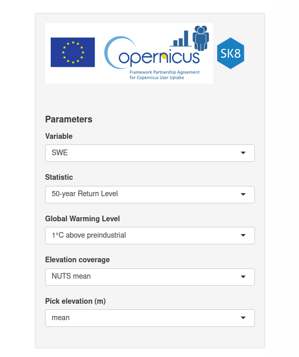
Variable “SWE” refers to the snow water equivalent. It represents the mass of water contained within the snow cover per surface unit. It is often expressed in kg.m-2, or in mm water equivalent - this is the unit used for the App. The snow load exerted by the snowpack on the underlying ground can directly be obtained by multiplying the SWE value by g (=9.8XXX) and is expressed in N.m-2 or Pa. The Statistic “50-year return level” is the key snow load indicator used for Eurocode safety standards. Under stationary conditions, it represents the value of the variable (SWE in our case) to be exceeded every 50 years on average. Similarly, there is a probability of 0.02 that the 50-year return level is exceeded each year.

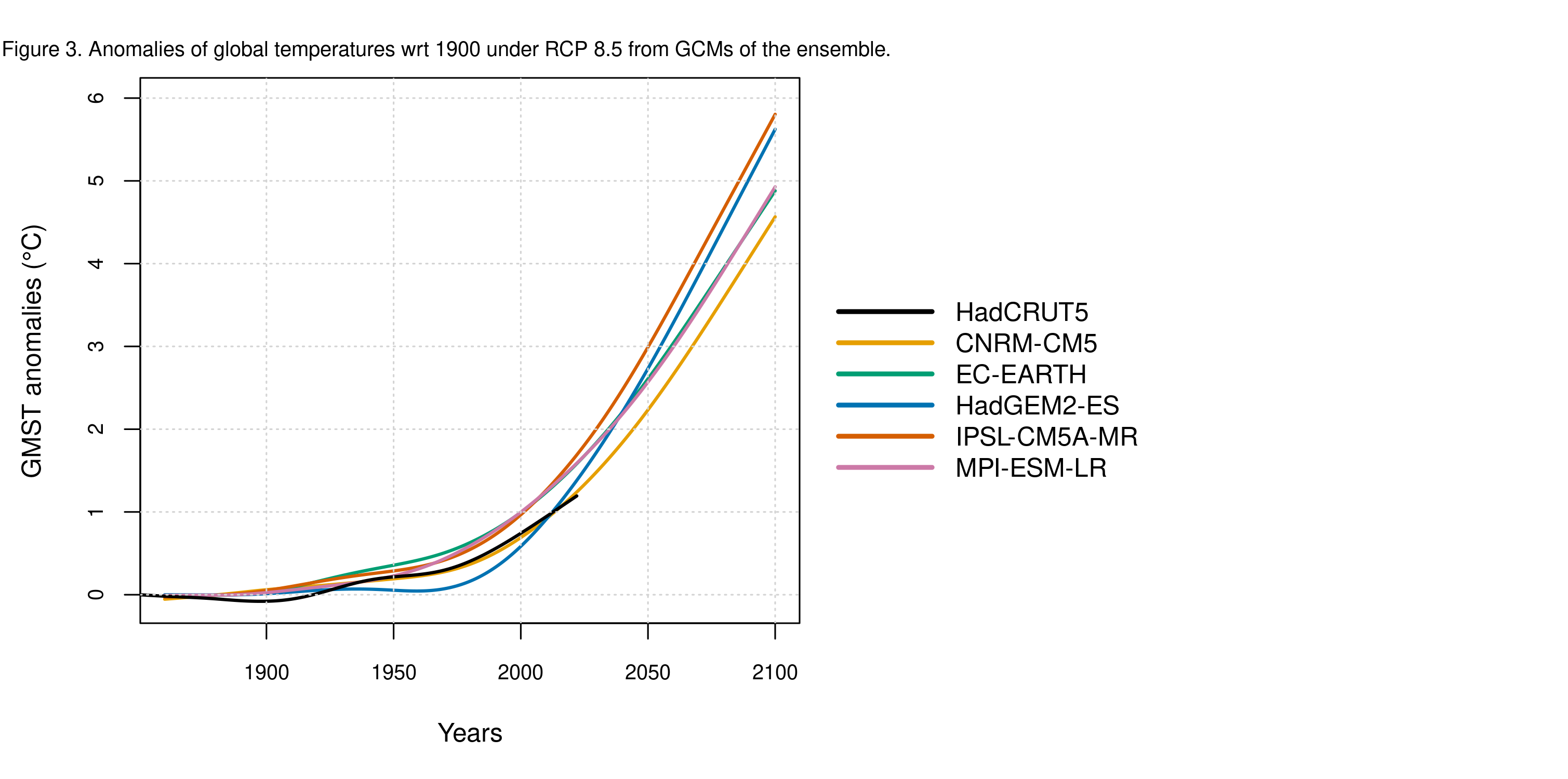
The Global Warming Level option “1°C above preindustrial” refers to the period on which the global mean temperature anomaly is 1 degree Celsius with respect to the preindustrial period 1860-1900 (GWL, see IPCC AR6 report1 ) . This corresponds to current climate conditions. The global mean temperature has undergone cubic spline smoothing prior to computing its anomaly. The option “3°C vs 1°C above preindustrial” refers to the comparison of two warming levels: the one on which the global mean temperature anomaly is 1 degree Celsius and the one on which the global mean temperature anomaly is 3 degree Celsius, both with respect to the preindustrial period 1860-1900.
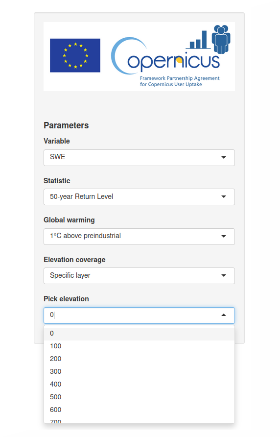
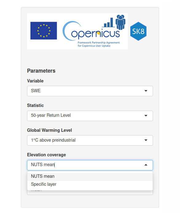
The Elevation coverage option refers to the filter that can be applied on NUTS-3 elevation (see section 4. for NUTS-3 definition). Either “NUTS mean” can be selected, and therefore information on all NUTS will be provided at their mean elevation. Otherwise, “Specific elevation” can be applied, which prompts the user to select a given elevation (see Pick elevation ). Available elevations range from “0 to 3300 m” , with 100 m steps (note that the elevation range differs according to the NUTS-3 regions).
4. Visual output: the map tab
The main Map tab (selected by default) shows the map corresponding to the options chosen.
a. Map scale
Information is given at NUTS-3 scale (Nomenclature des Unités Territoriales Statistiques2 at level 3), and on one or more altitude levels depending on the NUTS-3. NUTS-3 (hereafter called NUTS) borders are defined to mirror the territorial administrative division of EU countries, and thus provide a useful scale for local policies. In total, information for 1515 NUTS is provided.
b. Map properties
The map is built based on Pseudo-Mercator projection. OpenStreetMap is used as a basemap. The zooming level is flexible and can be adjusted by the user with the mouse scroll wheel or zooming button.
c. Color ramps
Two color scales are built. The one for relative values of SWE 50-year return levels is stable and goes from -100% to 160%, with one color per 20% interval. The color scale for absolute values is adjusted to the data, which rely on the user choice of elevation (being either the mean elevation, or a specific value).
d. Click on and pop-ups
When the user clicks on the geometry of any NUTS, relevant information is displayed as a pop-up: the NUTS (or region) name, the altitude on which information is provided (in meter), the absolute or relative value of 50-year return level (either in millimeter or percentage), and the uncertainty interval with units similar to the value’s - derived from quantiles 5% and 95% computed on bootstrapped values (see Data & Method ).
5. File output
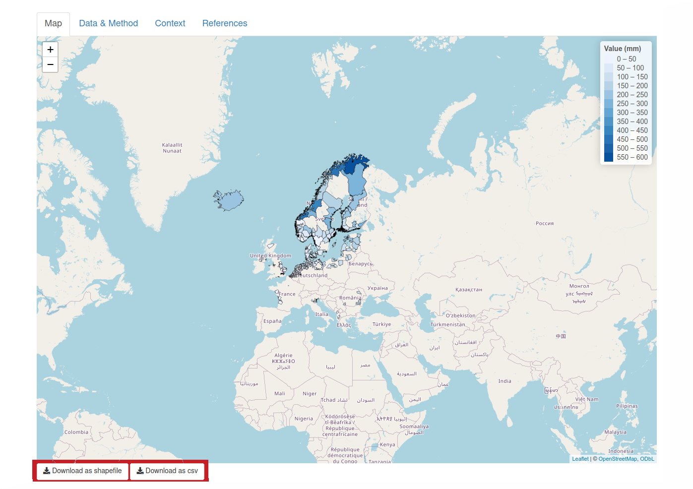
Two click on buttons are displayed below the map. It enables direct download of the data depicted on the current map - as filtered by the user. Each button corresponds to a format type, either .csv or .shp. As an example, the shapefile folder for set up global warming on 1°C anomaly, on NUTS mean elevation, is called “RL1degre_mean” (respectively “RL3vs1degre_100” for the relative value of 3°C vs 1°C on 100m elevation, etc…). Within each folder, the four files are simply called RL_1.* if global warming was set up on 1°C anomaly (respectively RL_3vs1.* if global warming was set up at 3°C vs 1°C). The downloaded csv file is named in a similar way to the shapefile folder introduced above, with an extra “.csv” suffix. One should note that the column names of the downloaded shapefiles are shorten: 'Val' refers to the value of return level, and 'Cni' to the associated confidence interval.
6. Other tabs
Ancillary information regarding the science behind the data shown is displayed on the other tabs. Data & Method gives details about the MTMSI data set used and the detailed method to provide return level outputs depicted on the maps. Context places the application within the SnowLoads project, giving an overview of the reason to be and purposes of the application. Lastly, Reference gathers the main scientific papers describing the data and methods used to produce the results depicted on the application.
7. Code and storage
The application has been developed with R. Among others, the Shiny and Leaflet packages have been used as they provide tools for interactive mapping. The application and data used to compute the maps are stored online in a storage called ForgeMIA which is managed by a team of INRAE affiliated computer scientists. The application is accessible under this link.
8. Acknowledgements
The authors of the present application thank the ForgeMIA team from INRAE for providing storage and support, enabling the app to be maintained and shared with stakeholders and scientists.
Data sets used
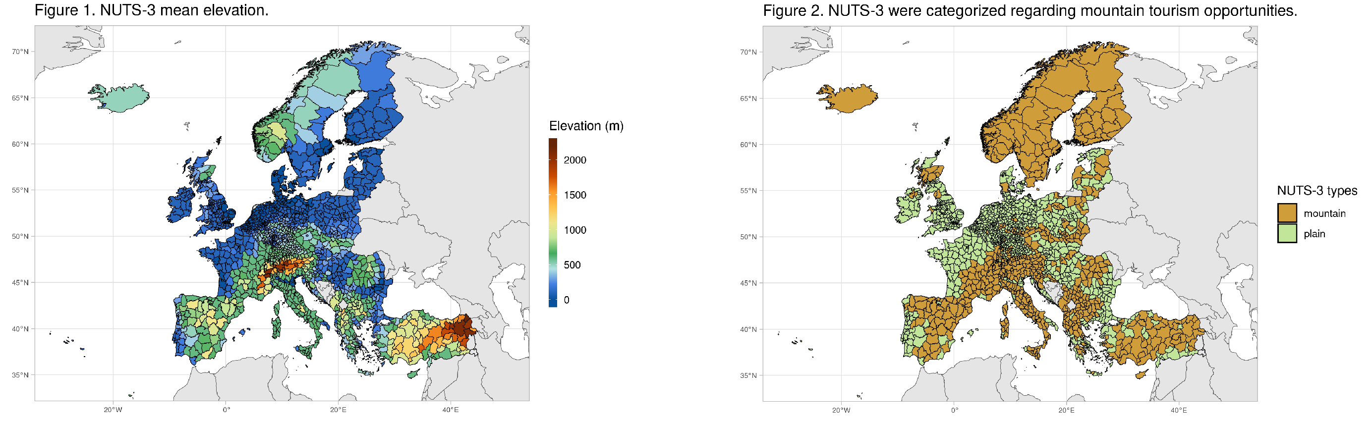
This portal uses data from the C3S Mountain Tourism Meteorological and Snow Indicators3 , which provides a set of snow related indicators based on the UERRA reanalysis and EURO-CORDEX projections at NUTS-3 (Nomenclature des Unités Territoriales Statistiques Indicators2 , 2013 and 2016 mixed version) level, by steps of 100 m elevation. In mountainous areas, the data is provided for several elevation steps, while for non-mountainous areas the data is provided at the mean elevation of the NUTS-3 (see Figure 1 and Figure 2). Here we use the annual SWE maximum (over each hydrological year, from August to July). The ADAMONT method4 was used to adjust the EURO-CORDEX GCM/RCM pairs using the UERRA 5.5 km reanalysis as an observation reference5 . Altogether, this projection ensemble comprises 20 future climate change scenarios for the 21st century (9 GCM/RCM pairs for RCP4.5 and RCP8.5, including 2 for RCP2.6).
Estimating 50-year return levels
We briefly present the method, detailed in Evin et al.6 , to estimate changes in extreme snow load (50-year return levels) in Europe as a function of global warming levels
Absolute valuesWe adjust different non-stationary models on SWE maxima. For each projection obtained with the emission scenario RCP8.5, the parameters of the different candidate distributions are dependent of the warming level of the GCM of the corresponding projection. For each GCM, the warming level is the anomaly of the global mean temperature with respect the preindustrial period 1860-1900, which has been smoothed using a cubic spline (see Figure 3). For each simulation chain (RCP8.5/GCM/RCM): (1) If there are less than 10% of non-zero SWE maxima, we no dot try to fit a distribution (insufficient data). (2) If there is at least one zero SWE maxima, we consider a discrete-continuous mixed distribution with a probability mass in zero and a continuous distribution (Exponential, Gamma, or Inverse-Gamma) for non-zero values. All parameters are considered to evolve linearly with the warming level (a logit transformation is applied to the parameter corresponding to the probability of having a zero values - the scale parameter σ and location parameter µ may also follow a transformation depending on the distribution). (3) Otherwise, if there is no zero SWE maxima, different continuous distributions are considered: Gamma, Generalized Gamma, Gumbel or GEV distribution7,8 (generalized extreme value). The shape parameter ξ is considered constant, the scale parameter σ and location parameter µ are considered to evolve linearly with the warming level (after potential transformation, regarding the distribution). For cases (2) and (3) we then select the best non-stationary model according to the AIC criteria. The 50-year return level estimation for each NUTS/altitude couple is taken as the mean over the 9 return levels obtained with the different simulation chains - distribution parameters being set to the desired warming level.
 Relative differences
Based on the results obtained through the method above, we computed the relative difference in return levels values between 1 degree and 3 degrees of global warming.
Confidence intervalThe confidence intervals express the uncertainty of the absolute and relative SWE values that have been computed. We assess two types of uncertainty. The first source of uncertainty corresponds to the sampling uncertainty. Indeed, the parameters of the different models are estimated using a limited amount of data, and this uncertainty is quantified using a non-parametric bootstrap method9 . 100 bootstrap estimates of 50-year return levels are provided for each simulation chain. The second type of uncertainty corresponds to the model uncertainty, i.e. the fact that different climate models lead to different future climate conditions. This second type of uncertainty is assessed using different simulating chains. An overall estimate of these two uncertainties is provided by the quantiles 0.05 and 0.95 of the 100 × 9 estimates. The difference between these two quantiles summarizes the magnitude of the uncertainties, and define the confidence intervals.
The FPCUP “Snowloads” project
Extreme snow fall and snow loads are challenging natural hazards in mountain areas and in lowlands. While both winter and summer are projected to become warmer throughout Europe, extreme precipitation is projected to increase throughout Europe10,11,12,13,14 . However, how the combination of temperature increase and extreme precipitation increase translates into changes in maximum annual amount of snow on the ground depends on location and elevation. As part of the “SNOWLOADS” project of Framework Partnership Agreement on Copernicus User Uptake (FPCUP), this portal provides information about past and future 50-year return level estimations of maximum annual snow mass, as it is key factor of Eurocodes infrastructure safety standards. The maximum annual snow mass, also referred to as the maximum annual snow water equivalent (SWE), expressed in kg/m2 (equivalent to mm water equivalent), is directly related to the snow load: the latter is obtained by multiplying SWE values by the gravity of Earth, typically 9.8 m/s2 .
For more information about FPCUP Snowloads click here .
The C3S application
The FPCUP SNOWLOADS application of Copernicus Climate Change Service (C3S) provides direct access to snowload extreme values under past and future climate in Europe, based on datasets of regional reanalyses and regional climate projections gathered through Copernicus. It enables users to visualize regional data depending on elevation and location ( see Data & Method ). The current portal is for demonstration only, and may later be implemented directly on a Copernicus-hosted portal.
1. IPCC, 2018. IPCC special report on the impacts of global warming of 1.5 °C above pre-industrial levels and related global greenhouse gas emission pathways, in the context of strengthening the global response to the threat of climate change, sustainable development, and efforts to eradicate poverty. y [V. Masson-Delmotte, P. Zhai, H. O. Pörtner, D.Roberts, J. Skea, P.R. Shukla, A. Pirani, W. Moufouma-Okia, C. Péan, R. Pidcock, S. Connors, J. B. R. Matthews, Y. Chen, X. Zhou, M. I. Gomis, E. Lonnoy, T. Maycock, M. Tignor, T. Waterfield (eds.)]. URL: http://www.ipcc.ch/report/sr15/. 151pp.
2. Eurostat NUTS, URL: https://ec.europa.eu/eurostat/fr/web/nuts/publications
3. S. Morin, R. Samacoits, H. Francois, C. M. Carmagnola, B. Abegg, O. Cenk Demiroglu, M. Pons, JM. Soubeyroux, M. Lafaysse, S. Franklin, G. Griffiths, D. Kite, A. Amacher Hoppler, E. George, C. Buontempo, S. Almond, G. Dubois and A. Cauchy, “Pan-european meteorological and snow indicators of climate change impact on ski tourism”, Climate Services , vol. 22, pp.100215, Apr. 2021.
4. D. Verfaillie, M. Deque, S. Morin, and M. Lafaysse, “The method ADAMONT v1.0 for statistical adjustment of climate projections applicable to energy balance land surface models”, Geoscientific Model Development , vol.10, no.11, pp.4257-4283, Nov. 2017.
5. C. Soci, E. Bazile, F. Besson, and T. Landelius, “High-resolution precipitation reanalysis system for climatological purposes”, Tellus A: Dynamic Meteorology and Oceanography , vol. 68, no. 1, pp.29879, Dec. 2016, Publisher: Taylor & Francis eprint: https://doi.org/10.3402/tellusa.v68.29879.
6. G. Evin, E. Le Roux, E. Kamir, S. Morin, “Estimating changes in extreme snow load in Europe as a function of global warming levels”, Cold Regions Science and Technology , vol. 231, Mar. 2025, eprint: https://doi.org/10.1016/j.coldregions.2025.104424
7. R. A. Fisher and L. H. C. Tippett, “Limiting forms of the frequency distribution of the largest or smallest member of a sample”, Mathematical Proceedings of the Cambridge Philosophical Society , vol. 24, no. 2, pp. 180–190, Apr. 1928, Publisher: Cambridge University Press.
8. B. Gnedenko, “Sur La Distribution Limite Du Terme Maximum D’Une Serie Aleatoire”, The Annals of Mathematics , vol. 44, no. 3, pp. 423, July 1943.
9. B. Efron and R. Tibshirani, “An Introduction to the Bootstrap (1st ed.)”, Chapman and Hall/CRC. , 1994
10. F. Giorgi and P. Lionello, “Climate change projections for the Mediterranean region”, Global and Planetary Change , vol. 63, no. 2, pp. 90–104, Sept. 2008.
11. D. Jacob, J. Petersen, B. Eggert, A. Alias, O. Bøssing Christensen, L. M. Bouwer, A. Braun, A. Colette, M. Deque, G. Georgievski, E. Georgopoulou, A. Gobiet, L. Menut, G. Nikulin, A. Haensler, N. Hempelmann, C., K. Keuler, S. Kovats, N. Kroner, S. Kotlarski, A. Kriegsmann, E. Martin, E. van Meijgaard, C. Moseley, S. Pfeifer, S. Preuschmann, C. Radermacher, K. Radtke, D. Rechid, M. Rounsevell, P. Samuelsson, S. Somot, JF. Soussana, C. Teichmann, R. Valentini, R. Vautard, B. Weber, and P. Yiou, “EURO-CORDEX: new high-resolution climate change projections for European impact research”, Regional Environmental Change , vol. 14, no. 2, pp. 563–578, Apr. 2014.
12. S. Russo, J. Sillmann, and E. M. Fischer, “Top ten European heatwaves since 1950 and their occurrence in the coming decades”, Environmental Research Letters , vol. 10, no. 12, pp. 124003, Nov. 2015, Publisher: IOP Publishing.
13. E. Kjellstrom, G. Nikulin, G. Strandberg, O. B. Chri-tensen, D. Jacob, K. Keuler, G. Lenderink, E. van Meijgaard, C. Schar, S. Somot, S. L. Sørland, C. Teichmann , and R. Vautard, “European climate change at global mean temperature increases of 1.5 and 2 degree Celsius above pre-industrial conditions as simulated by the EURO-CORDEX regional climate models”, Earth System Dynamics , vol. 9, no. 2, pp. 459–478, 2018.
14. J. Hesselbjerg Christensen, M. A. D. Larsen, O. B. Christensen, M. Drews, and M. Stendel, “Robustness of European climate projections from dynamical downscaling”, Climate Dynamics , vol. 53, no. 7, pp. 4857–4869, Oct. 2019.